GMPL/glpk basics
An overview of tools and languages for (MI)LP problems, and a bit of introduction to GLPK and GMPL
- Prerequisites Linear Programming: first steps
(MI)LP description languages and solvers
Since MILP and LP models are widely used in practice, the algorithms solving them are well implemented already. Thus, there is no need to implement the simplex algorithm ourselves. Thruthfully, it is better if one doesn't do that unless it is for getting a bit of coding practice. State-of-the-art solvers are rather complex, and there are small but significant details (like floating point rounding), that have to be addressed to produce a stable solver, and even if that is done, the result will be nowhere close to the efficiency of the solvers mentioned below. The solvers in the list use a lot of theoretical accelerations (e.g. LU decomposition), implementational "tricks" (e.g. Sparse representation), and a lots of heuristic accelerations.
There are several choices for solving MILP/LP problems. Some are listed below, with some information about them.
| Solver | License | Problem classes |
|---|---|---|
| lp_solve | LGPL | MILP |
| GLPK | GPL | MILP |
| COIN-OR CLP | EPL | LP |
| COIN-OR CBC | EPL | MILP |
| Gurobi | Proprietary - Gurobi Optimization | MIQP i |
| CPLEX | Proprietary - IBM | MIQP i |
| LINGO | Proprietary - Lindo systems inc. | MILP, MINLP |
As this selective list shows, there are a lot of options to chose from, and there is even more.
Regarding performance, the proprietary tools outperform the open source alternatives by far. Among the open source solutions, the COIN OR project can be considered the fastest one. Ultimately, the situation dictates, which one you should apply. For example, I use (or would use)
- the standalone solver of GLPK for teaching purposes, as it is really simple to install/use, and it is freely available.
- the API of COIN OR in scientific software, that need to solve MILP problems as subproblems.
- Gurobi/CPLEX and COIN OR CBC for comparison purposes in scientific papers.
- Gurobi/CPLEX in an industrial environment where efficiency is key.
If the solver is selected, you can either use its API from your code, or use the standalone solver with a model file. Different tools support API for different languages, but let us focus on the second option for now. There is a wide variety of languages for describing MILP models, and the tools usually support several of them. The table below shows some examples.
| Format name | Usual extension | Description, notes |
|---|---|---|
| AMPL | .mod .dat .run |
A Mathematical Programming Language. Very general and multipurpose language, widely used. |
| GMPL | .mod .dat |
GNU Mathematical Programming Language. Subset of AMPL, default for GLPK. |
| MPS | .mod .dat |
Mathematical Programming System. Old format, most solvers can use it as a legacy option. |
| GAMS | TODO |
General Algebraic Modeling System. A file format, an interpreter, an IDE and an API for solvers. |
| CPLEX | .lp |
Default format for CPLEX, widely accepted by other solvers. |
| Lingo | .lng |
The format used by only LINGO. |
Below You can see the same example in a few different formats for comapirson.
\[x+2\cdot y\le 15\] \[3\cdot x+y\le 20\]
\[x+y \to max\]
* Problem:    helloworld
* Class:      LP
* Rows:       3
* Columns:    2
* Non-zeros:  6
* Format:     Fixed MPS
*
NAME          hellowor
ROWS
 L  R0000001
 L  R0000002
 N  R0000003
COLUMNS
    x         R0000001             1   R0000002             3
    x         R0000003             1
    y         R0000001             2   R0000002             1
    y         R0000003             1
RHS
    RHS1      R0000001            15   R0000002            20
ENDATA
* Problem:    helloworld
* Class:      LP
* Rows:       3
* Columns:    2
* Non-zeros:  6
* Format:     Free MPS
*
NAME helloworld
ROWS
 L Constraint1
 L Constraint2
 N Objective
COLUMNS
 x Constraint1 1 Constraint2 3
 x Objective 1
 y Constraint1 2 Constraint2 1
 y Objective 1
RHS
 RHS1 Constraint1 15 Constraint2 20
ENDATA
\* Problem: helloworld *\

Maximize
 Objective: + x + y

Subject To
 Constraint1: + x + 2 y <= 15
 Constraint2: + 3 x + y <= 20

End
var x>=0;
var y>=0;

s.t. Constraint1:
  x + 2*y <= 15;

s.t. Constraint2:
  3*x + y <= 20;

maximize Objective: x+y;
MODEL:
MAX = X + Y;
X >= 0;
Y >= 0;
X + 2 * Y <= 15;
3 * X + Y <= 20;
END
--wmps, --wfreemps, --wlp options.
GMPL basics
As it was discussed previously, the model can be partitioned into three parts: variable declarations, constraints, and the objective function. We will follow this order to introduce the basic syntactic elements of GMPL. You can find a detailed reference of the GMPL format if You download the package from the website of GLPK.
Variables
Variables can be defined with the var keyword, that should be followed by the name of the variable, restrictions on the domain, and finally a semicolon.
Some examples:
| Mathematical notation | GMPL code |
|---|---|
| \(x\in[0,\infty[\) | var x>=0; |
| \(x\in[0,8]\) | var x>=0,<=8; |
| \(y\in\{0,1\}\) | var y binary; |
| \(y\in\mathbb{Z}\) | var y integer; |
| \(y\in\mathbb{N}\) | var y integer >=0; |
Constraints
Constraints are written in the form of s.t. CNAME: LHS OP RHS; where CNAME is an expressive name for the constraint, LHS,RHS are the left- and right-hand side of the inequality/equasion respectively, separated by a comparison operator, that could be either <=,>= or =.
The name of the constraint does not hold any importance to the solver, it is just an identifier, that also helps to make the code more human-readable and maintainable.
Also, mind the colon for separating the name and the constraint, and a semicolon closing the statement. Some examples:
| Mathematical notation | GMPL code |
|---|---|
| \(x_1+x_2\le 10\) | s.t. SumBound: x1+x2 <= 10; |
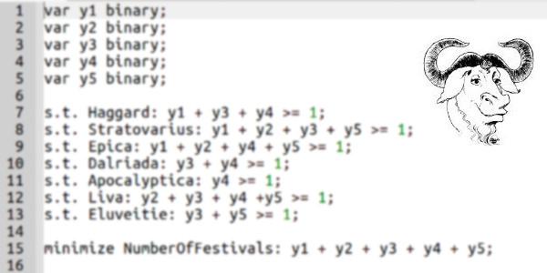
| \(y_1+y_2+y_3+y_5\ge 1\) | s.t. Stratovarius: y1+y2+y3+y5 >= 1; |
| \(1 \cdot x_{KF} + 2\cdot x_{NF} +1\cdot x_{HL} = 1000\) | s.t. UseUpAllTheWine: 1*xKF+2*xNF+1*xHL = 1000; |
Objective function
The syntax for the objective function is very similar to that of the constraint: [minimize|maximize] ONAME: EXPRESSION;, where ONAME is a name assigned to the objective function, and the EXPRESSION is the linear expression for it.
Again, mind the colons, semi-colons.
Two examples:
| Mathematical notation | GMPL code |
|---|---|
| \( y_1+y_2+y_3+y_4+y_5 \to min\) | minimize VisitedFestivals: y1+y2+y3+y4+y5; |
| \( 110 \cdot x_{KF} + 200 \cdot x_{NF} + 120 \cdot x_{HL} \to max\) | maximize TotalIncome: 110*xKF+200*xNF+120*xHL; |
We are ready to solve our motivational examples, but let's see how we can make the solver find the optimal solution for the models we implement in GMPL.
Using GLPK
The examples here will assume, that You run glpsol from the command line.
- Always save Your model with the
.modextension, otherwise the editor will not consider it as a GMPL file. - Before clicking on Go, or pressing F5, make sure to check the "Generate output file on go" option in the Tools menu.
The basic command to solve a file is glspsol -m model.m -o output.txt.
This will read the model from model.m, write the results to output.txt, and display some info on the standard output whilst doing it.
If You run the above command on the simple example used above for demonstrating the different file formats, You will get this in the terminal:
bash$ glpsol -m helloworld.m -o output.txt
GLPSOL: GLPK LP/MIP Solver, v4.57
Parameter(s) specified in the command line:
 -m helloworld.m -o output.txt
Reading model section from helloworld.m...
helloworld.m:10: warning: unexpected end of file; missing end statement inserted
10 lines were read
Generating Constraint1...
Generating Constraint2...
Generating Objective...
Model has been successfully generated
GLPK Simplex Optimizer, v4.57
3 rows, 2 columns, 6 non-zeros
Preprocessing...
2 rows, 2 columns, 4 non-zeros
Scaling...
 A: min|aij| =  1.000e+00  max|aij| =  3.000e+00  ratio =  3.000e+00
Problem data seem to be well scaled
Constructing initial basis...
Size of triangular part is 2
*     0: obj =  -0.000000000e+00 inf =   0.000e+00 (2)
*     2: obj =   1.000000000e+01 inf =   0.000e+00 (0)
OPTIMAL LP SOLUTION FOUND
Time used:   0.0 secs
Memory used: 0.1 Mb (102269 bytes)
Writing basic solution to 'output.txt'...
bash$
There are a bunch of things here, familiar ringing words, like "Preprocessing", but for now, we will only focus on the line with all capitals: OPTIMAL LP SOLUTION FOUND. This line indicates, that the problem has been solved to optimality.
For MILP models, the message would be a little different: INTEGER OPTIMAL SOLUTION FOUND.
If we see other messages indicating that no feasible solution were found, or the solution is unbounded, than we have probably over- or underconstrained the problem, respectively.
More about that later, let's see, what is in the generated output.txt file.
Problem:    helloworld
Rows:       3
Columns:    2
Non-zeros:  6
Status:     OPTIMAL
Objective:  Objective = 10 (MAXimum)

   No.   Row name   St   Activity     Lower bound   Upper bound    Marginal
------ ------------ -- ------------- ------------- ------------- -------------
     1 Constraint1  NU            15                          15           0.4
     2 Constraint2  NU            20                          20           0.2
     3 Objective    B             10

   No. Column name  St   Activity     Lower bound   Upper bound    Marginal
------ ------------ -- ------------- ------------- ------------- -------------
     1 x            B              5             0
     2 y            B              5             0

Karush-Kuhn-Tucker optimality conditions:

KKT.PE: max.abs.err = 0.00e+00 on row 0
        max.rel.err = 0.00e+00 on row 0
        High quality

KKT.PB: max.abs.err = 0.00e+00 on row 0
        max.rel.err = 0.00e+00 on row 0
        High quality

KKT.DE: max.abs.err = 0.00e+00 on column 0
        max.rel.err = 0.00e+00 on column 0
        High quality

KKT.DB: max.abs.err = 0.00e+00 on row 0
        max.rel.err = 0.00e+00 on row 0
        High quality

End of output
Again, there is plenty of information here as well, but we will only need specific lines for now.
First, the fifth line with Status: OPTIMAL indicates again, that everything went well, and we have found an optimal solution.
The line below that tells us, what that optimal solution is.
Here, the word "Objective" appears twice, which seems buggy.
But this is just a coincidence, as the first appearance is burned in the solver, and the second is the name that we gave to our objective function, which happened to be "Objective" as well for this simple problem.
It is good to know the quality of the optimal solution (10 in this case), but in general, we also want to know, Activity column of the second table.
In this case, we can see, that the optimal solution is achieved by setting both x and y to 5.