• Prerequisites
Motivational example: festivals Motivational example: fröccs

Modeling in general

Modeling is a technique used in many fields with different purposes, such as simulation, planning, and of course, optimization. A model is essentially a simplified version of something real, which is easier, cheaper to deal with. A model is not necessarily a mathematical one, a mock-up can be thought of as a physical model. On this site, however, the word model will always refer to a mathematical model, unless specified otherwise.

There are many things, that could serve as a model. The simplest ones are thought in secondary school physics classes, e.g., \( v=\frac{s}{t} \), where v denotes the average velocity if the distance s is covered within t time. This model is a simple equation between 3 variables. Other models may employ different mathematical structures, such as graphs. In this course, we will focus on algebraic models as discussed below.

It is important to note, that in most of the cases, a model is only a "simplification" of a real life phenomena. Usually, the model disregards some parameters, that may influence the behavior of a system. In the above example, it was assumed, that the object moved along a straight line. When a real life problem emerges, the modeler has a great responsibility in selecting the parameters to be included into the model, and the level of detail, how they are represented.

This can be very well presented on the evolution of GPS navigation tools. The basic problem is simple, we want to get from point A to point B as fast as possible.

1. The simplest approach to apply is to find the shortest path between the locations. This could be done easily, if the weighted graph of the road network is available.
2. A bit more advanced approach would be, if we took into account the speed limit on each part of the road, and replace the distances in the graph with the minimal travel time needed. Computationally speaking, this approach requires the same resources, however, more input data is required.
3. Most of the modern navigation systems, that run on devices with internet connection go a step further, and use real time traffic data to consider while planning a trip.

We could even go further by including weather data, road conditions, characteristics of the driver, etc. As we include more and more parameters, the model becomes more and more accurate, but also more difficult to handle.

Later on, we will not focus on this very first step of modeling, and we will assume, that these decisions are already made, and we just have to construct and solve the appropriate mathematical model.

Model for the Fröccs example

Let us assume, that we have a solution. Not necessarily optimal, but any solution. The solution entails, how much we sell from different kinds of beverages. Let \(x_{KF}\) denote the number of portions we sell from kisfröccs, \(x_{NF}\) the number of portions for nagyfröccs, and so on.

Based on these values, we can calculate, how much wine was needed for this solution in a simple way. For \(x_{KF}\) portions of kisfröccs \(x_{KF}\cdot 1\) dl of wine is needed. Similarly, \(x_{NF}\cdot 2\) dl of wine had to be used for \(x_{NF}\) portions of nagyfröccs. Following this logic, the total amount of wine used in deciliters is: \[1 \cdot x_{KF} + 2 \cdot x_{NF}\ + 1 \cdot x_{HL} + 3 \cdot x_{HM} + 2 \cdot x_{VHM} + 9 \cdot x_{KrF} + 1 \cdot x_{SF} + 6 \cdot x_{PF}\]

The stock for wines is 100 litres = 1000 deciliters, so, whatever those values are, the following inequality must hold in a good solution: \[1 \cdot x_{KF} + 2 \cdot x_{NF}\ + 1 \cdot x_{HL} + 3 \cdot x_{HM} + 2 \cdot x_{VHM} + 9 \cdot x_{KrF} + 1 \cdot x_{SF} + 6 \cdot x_{PF} \le 1000\]

A very similar constraint could be constructed for the soda as well: \[1 \cdot x_{KF} + 1 \cdot x_{NF}\ + 2 \cdot x_{HL} + 2 \cdot x_{HM} + 3 \cdot x_{VHM} + 1 \cdot x_{KrF} + 9 \cdot x_{SF} + 3 \cdot x_{PF} \le 1500\]

If the values for \(x_{KF}, x_{NF}, \dots\) are selected from the \([0,\infty[\) interval so, that the two inequalities above are satisfied, then that solution is feasible and good. We have now a simple algebraic model for the restrictions of the model. The only thing missing is to express our objective.

Similarly to the wine and soda usage, the profit attained with such a plan is: \[110 \cdot x_{KF} + 200 \cdot x_{NF}\ + 120 \cdot x_{HL} + 260 \cdot x_{HM} + 200 \cdot x_{VHM} + 800 \cdot x_{KrF} + 200 \cdot x_{SF} + 550 \cdot x_{PF}\] And this is, what we want to maximize.

Now, if we put together everything, we get:

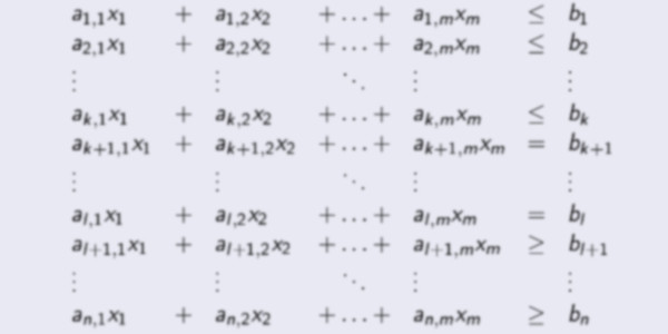
This mathematical description of the problems restrictions, goals, decision flexibilities adheres the rules of a Linear Programming model, or LP for short:

1. There are a finite number of variables
2. The domain of each variable is a continuous interval
3. There are a finite number of constraints
4. The left hand side (LHS) of each constraint is a linear expression of the variables
5. The relation in each constraint is either \(\le\),\(=\), or \(\ge\)
6. The right hand side (RHS) of each constraint is a constant Note
7. The objective function is a linear expression of the variables, that can be either maximized or minimized

Mathematical models that meet the above conditions are LP models, and can be solved to optimality efficiently (computational time is bounded by a polinomial function of the number of variables) by a simplex algorithm variant or interior point method.

Model for the Festival example

Let's try to create a model similar to the previous one for the festival example. First, observe the relation between the parts of the problem description and the parts of the mathematical model.

In the LP model above, the variables represented the decisions that we can make, i.e., a flexibility of a problem. Each possible option for a decision is encoded by a value in the domain of the corresponding variable, and vica-versa. The restrictions of the problem description were expressed via constraints. Finally, the objective function modeled our goal.

Problem definition		Linear Programming model
Decision	\(\iff\)	Variable
Option for decision	\(\iff\)	Value of the variable
Restriction	\(\iff\)	Constraints
Goal	\(\iff\)	Objective function

Let's construct the model along these lines in three simple step:

Step 1: variables

For the festival example, the decisions we can make is, whether we go to a festival or not. Let's represent that with variables \(y_1,y_2,y_3,y_4\) and \(y_5\).

Now, we have to define the domain of each variable, and assign a "meaning" (decision option) to each possible value. In this case, the possible outcome for each decision is either that we go to that particular festival or not. Thus, the domain must have two elements. Theoretically, we could choose any two numerical value, however, it is logical (and it will be useful later) to have the following assignments:

\(y_n=1\)

We will go to the \(n\)-th festival

\(y_n=0\)

We will not go to the \(n\)-th festival

Step 2: constraints

If the variables and the value assignments are selected appropriately, deriving the equations is often rather straightforward, like for the fröccs example above. Sometimes it is a bit more tricky, like in this case.

First we have to identify our restrictions. In this case the only restriction is: we have to see all of our favorite bands at least once. Truthfully, that actually means 7 separate conditions for the 7 bands.

Sticking to my favorites, we know that we have to go to at least one of festivals 1,3 and 4 in order to see Haggard. Translating that to our variables: at least one of \(y_1,y_3,y_4\) must take the value of 1. So we have to construct a constraint, that evaluates to true if and only if at least one of these variables are 1.

Try to figure out a (linear) constraint like that yourself before scrolling further!

\(y_1\)	\(y_3\)	\(y_4\)	\(y_1+y_2+y_3 \ge 1 \)
0	0	0	\( 0 \not\ge 1\)
0	0	1	\( 1 \ge 1\)
0	1	0	\( 1 \ge 1\)
0	1	1	\( 2 \ge 1\)
1	0	0	\( 1 \ge 1\)
1	0	1	\( 2 \ge 1\)
1	1	0	\( 2 \ge 1\)
1	1	1	\( 3 \ge 1\)

Following this example, a similar constraint could be derived for all of the bands, e.g., for Stratovarius: \[ y_1 + y_2 + y_3 + y_5 \ge 1 \] for Dalriada: \[y_3 + y_5 \ge 1 \] The case of Apocalyptica is very special: \(y_4 \ge 1\), which basically sets \(y_4\) to 1. That is expected, as the 4th festival is the only one, where Apocalyptica performs.

Step 3: objective

Our objective is to go to as few festivals as possible. Using the \(y_n\) variables, we should somehow express the number of festivals that we visit. It is not difficult to see, that \(y_1+y_2+y_3+y_4+y_5\) does exactly that.

Finally, the whole model

Putting everything from above together:

Now, let's see, if this model adheres the rules of an LP model (above) or not:

1. There are a finite number of variables - 🗸
2. The domain of each variable is a continuous interval
3. There are a finite number of constraints - 🗸
4. The left hand side (LHS) of each constraint is a linear expression of the variables - 🗸
5. The relation in each constraint is either \(\le\),\(=\), or \(\ge\) - 🗸
6. The right hand side (RHS) of each constraint is a constant - 🗸
7. The objective function is a linear expression of the variables, that can be either maximized or minimized - 🗸

So, this is not an LP model, but something very similar. The only difference is, that (some of) the variables take their values from a discrete set. These types of problems are termed Mixed-Integer Linear Programming (MILP) problems. In these models some variables may take values from a continuous interval, some may take only discrete values, such as integers. Theoretically speaking, any kind of discrete set could be used for a variable, but usually only subsets of \(\mathbb{Z}\) are considered, and thus these are called as integer variables. It is very common, that this subset is \(\{0,1\}\), so this type of variables have their own name, binary variables. In our example, all of the variables are binary, and there are no other integer or continuous variables used.

MILP models are (computationally speaking) more difficult to solve. MILP solvers usually combine the simplex algorithm with some other technique, such as a Branch-and-Bound (B\&B) algorithm or Cutting-plane / Branch-and-Cut method. Speaking vaguely, the time (number of steps) required to solve a general MILP problem is an exponential function of the number of integer variables. This means, that after a certain number of variables, the problem becomes really hard, and practically unsolvable to optimality. The aforementioned tools will still provide a solution if the solver is shut down after a time limit, but the optimality of that solution is not guaranteed.

Note, that not all MILP models are difficult to solve. If, for example, the matrix of the coefficients in the model is totally unimodular, the problem can be solved in polinomial time, just as in the case for LP problems. A famous example is the Assignment problem, which can be solved efficiently by the Hungarian method. (The algorithm was developed by an american mathemtician, Harold W. Kuhn, who gave this name because the algorithm was based on the former works of two Hungarian mathematicians: Dénes Kőnig and Jenő Egerváry. The former is the author of the first graph-theory textbook.)

---